data-310-page

---

Project maintained by ecwydra Hosted on GitHub Pages — Theme by mattgraham

Lab 1

Question 1

What would be the most commonly used level of measurement if the variable is the temperature of the air?

1. interval – this is the answer
2. nominal
3. ratio
4. ordinal

Question 2

NaNs were replaced with 21.0.

# data handling imports
import numpy as np
import pandas as pd
from sklearn.impute import SimpleImputer

# import the csv file
data_2 = pd.read_csv('L1Data.csv')

# set the imputing configuration
imp_config = SimpleImputer(missing_values = np.nan, strategy = 'median')

# choose column for imputation
imp = imp_config.fit(data_2_noNaN[['Age']])

# replace NaNs in data_2_noNaN
data_2_noNaN[['Age']] = imp.transform(data_2_noNaN[['Age']]).ravel()

data_2_noNaN # row 12 and 20 replaced with 21.0

Question 3

In Bayesian inference the “likelihood” represents:

1. How probably is the new evidence under all possible hypotheses
2. How probably is our hypothesis given the data observations (the specific evidence we collected)
3. How probable is the data/evidence given that our hypothesis is true – this is the answer
4. How probable or frequent is our hypothesis in general

Question 4

The main goal of Monte Carlo simulations is to solve problems by approximating a probability value through carefully designed simulations.

This is true

Question 5

Assume that during a pandemic…

• 15% of the population gets infected with a respiratory virus
• 35% of the population have general respiratory symptoms
• 30% of those infected are asymptomatic

What is the probablity that someone who is symptomatic has the disease?

pop_infected = 0.15
pop_symptom = 0.35
pop_asymp = 0.30
pop_nasymp = 0.70

probability = ((pop_infected * pop_nasymp) / pop_symptom) * 100

probability # is 30.0

Question 6

A Monte Carlo simulation should never include more than 1000 repetitions of the experiment.

This is false

Question 7

One can decide that the number of iterations in a Monte Carlo simulation was sufficient by visualizing a Probability-Iteration plot and determining where the probability graph approaches a horizontal line.

This is true

Question 8

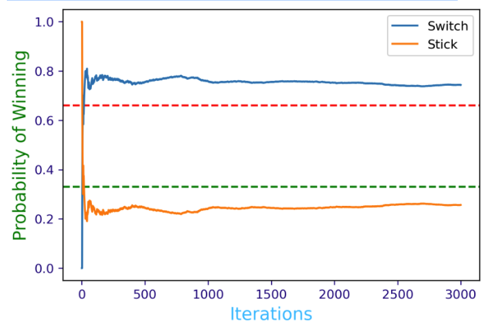
Assume we play a slightly bit different version of the original Monte Hall problem such as having four doors one car and three goats. The rules of the game are the same, the contestant chooses one door (that remains closed) and one of the other doors who had a goat behind it is being opened. The contestant has to make a choice as to stick with the original choice or rather switch for one of the remaining closed doors.

%matplotlib inline
%config InlineBackend.figure_format = 'retina'
import matplotlib as mpl
mpl.rcParams['figure.dpi'] = 150

import random
import matplotlib.pyplot as plt

doors = ["goat","goat", "goat", "car"]

# approximated results
switch_win_probability = []
stick_win_probability = []

plt.axhline(y=0.66, color='red', linestyle='--')
plt.axhline(y=0.33, color='green', linestyle='--')

def monte_carlo(n):

  switch_wins = 0
  stick_wins = 0

  for i in range(n):
     random.shuffle(doors)

     k = random.randrange(4)

     if doors[k] != 'car':
       switch_wins +=1

     else:
       stick_wins +=1

     switch_win_probability.append(switch_wins/(i+1))
     stick_win_probability.append(stick_wins/(i+1))

  plt.plot(switch_win_probability,label='Switch')
  plt.plot(stick_win_probability,label='Stick')
  plt.tick_params(axis='x', colors='navy')
  plt.tick_params(axis='y', colors='navy')
  plt.xlabel('Iterations',fontsize=14,color='DeepSkyBlue')
  plt.ylabel('Probability of Winning',fontsize=14,color='green')
  plt.legend()
  print('Winning probability if you always switch:', switch_win_probability[-1])
  print('Winning probability if you always stick to your original choice:', stick_win_probability[-1])

monte_carlo(3000)

Winning probability if you always switch: 0.7436666666666667 Winning probability if you always stick to your original choice: 0.25633333333333336

Graph of results:

Question 9

In Python one of the libraries that we can use for generating repeated experiments in Monte Carlo simulations is:

1. matplotlib
2. math
3. random – It’s this one
4. pandas

Question 10

In Python, for creating a random permutation of an array whose entries are nominal variables we used:

1. random.randint
2. random.uniform
3. random.shuffle – It’s this one
4. random.randrange